
01 / The case: a dose that starts to move
An automated dispenser applies an adhesive bead around the flange of an electronics housing before the cover is fitted. The team wants a consistent application: enough material for the intended joint, without uncontrolled excess entering nearby features when the housing is closed. The actual acceptable quantity must come from the product design, adhesive supplier guidance and validated assembly requirements.
A technician notices that the bead appears fuller during a later sampling check. That observation is useful, but appearance alone cannot establish whether the dispensing process changed. A slightly different viewing angle, bead path or surface condition can change what the application looks like. The team therefore monitors a defined, repeatable parameter: adhesive mass per dispense, measured in grams.
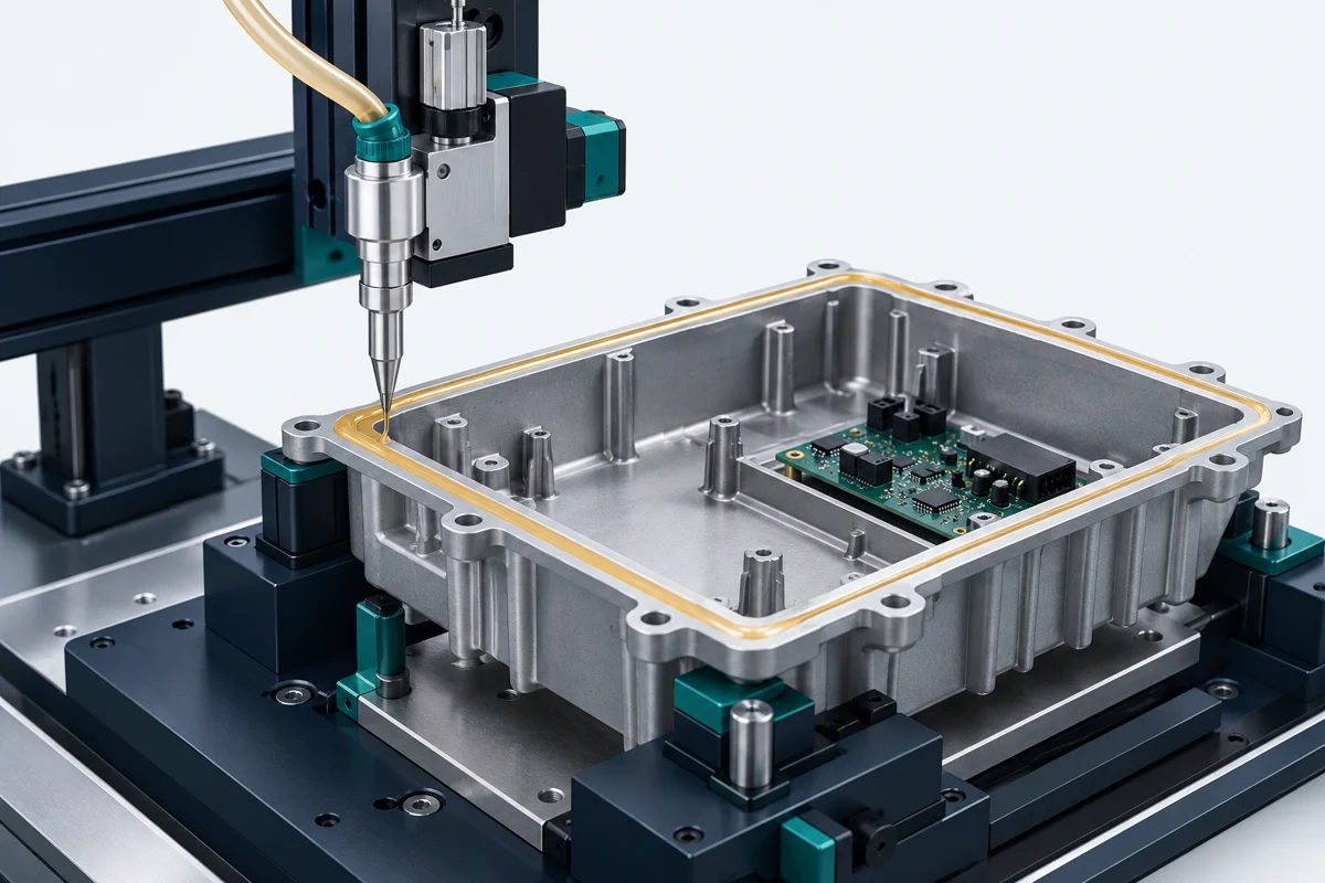
The question is concrete: did the dispenser continue delivering the same kind of dose throughout the sampling sequence, or did its average output change? Statistical process control helps answer that question by keeping the measurements in their collection order. It also separates a change in the process average from a change in the spread of consecutive dispenses.
02 / Define the measurement before collecting data
For this example, the operator collects each complete dispense cycle into a clean, tared container and weighs the net adhesive mass. The collection method must represent the production dispense cycle closely enough to be useful. A different nozzle path, dispense duration or back-pressure condition could make a collection test unrepresentative of the actual assembly operation.
Keep the weighing procedure consistent: use the same collection method, verify the balance according to the local procedure, record the tare correctly and avoid residue or material loss. Resolution and repeatability must be appropriate for the differences being investigated. A balance display showing extra decimals does not, by itself, establish measurement suitability.
Weighing the housing before and after dispensing is another possible method, provided the net difference can be measured reliably. It may avoid changing the dispense operation, but the much larger housing mass, fixture handling and weighing conditions can affect the result. Choose and validate the method for the process rather than switching methods halfway through the study.
Mass is an operational indicator here. It does not establish bead continuity, placement, curing or bond performance. Those characteristics may need their own inspection or process controls. A consistent total mass could still be distributed incorrectly around the housing.
03 / Collect rational subgroups, not a mixed bag of readings
The operator collects four consecutive dispenses every 30 minutes. Each group represents a short window under similar operating conditions. The four readings reveal short-term spread within that window. Comparing the subgroup averages shows how the process location behaves between sampling intervals.
Do not build a subgroup by selecting one reading from each of four different hours. That mixes between-time changes into the within-subgroup range and changes the meaning of the chart. Likewise, readings from different machines, nozzles or product recipes should not automatically be pooled as though they came from one consistent stream.
The 30-minute interval is an illustrative choice, not a universal recommendation. Set the frequency according to cycle time, consequences of a missed change, response time and known process dynamics. For a fast-changing process, half an hour may leave too much production between checks. For another process, a different interval or continuous monitoring may be appropriate.
Keep a small event log alongside the readings: timestamp, machine and nozzle identification, material lot, recipe, recent adjustments, interruptions and relevant environmental conditions. SPC provides a signal; the event history makes that signal easier to investigate.
04 / The six-subgroup dataset
The first five subgroup averages vary slightly around 10.00 g, from 9.990 to 10.010 g. At the sixth check, the average rises to 10.120 g. The individual readings and subgroup ranges also vary: a repeatable process does not deliver an identical value every cycle. These constructed teaching data include small fluctuations while keeping the later change easy to examine.
| Subgroup | Time | 1 | 2 | 3 | 4 | Average | Range |
|---|---|---|---|---|---|---|---|
| 1 | 08:00 | 9.99 | 10.02 | 10.00 | 9.99 | 10.000 | 0.030 |
| 2 | 08:30 | 9.99 | 10.04 | 10.00 | 10.01 | 10.010 | 0.050 |
| 3 | 09:00 | 9.97 | 10.01 | 9.98 | 10.00 | 9.990 | 0.040 |
| 4 | 09:30 | 9.98 | 10.04 | 10.00 | 10.00 | 10.005 | 0.060 |
| 5 | 10:00 | 9.97 | 10.02 | 9.99 | 10.00 | 9.995 | 0.050 |
| 6 | 10:30 | 10.10 | 10.13 | 10.11 | 10.14 | 10.120 | 0.040 |
Download the measurement table (CSV). The time labels are part of this illustrative sampling schedule.
For subgroup 1, the average is (9.99 + 10.02 + 10.00 + 9.99) / 4 = 10.00 g. Its range is 10.02 − 9.99 = 0.030 g. Subgroup 6 gives an average of 10.12 g and a range of 10.14 − 10.10 = 0.040 g. The sixth group sits above the earlier readings, but its range remains within the 0.030–0.060 g spread observed in the earlier groups.
05 / Read the two charts together
The R chart tracks each subgroup’s range. In this dataset, the ranges fluctuate between 0.030 and 0.060 g, and none crosses a range control limit. That is evidence of no immediate range-limit violation in this short example; it is not proof that the process has established long-term control.
R chart / within-subgroup spread
The X̄ chart tracks the six subgroup averages. The first five fluctuate near 10.00 g; the sixth is 10.12 g. That last average exceeds the calculated upper control limit. The paired reading is therefore specific: short-term spread varies within the provisional range limits, while the process average shows a limit-crossing signal at subgroup 6.
X̄ chart / subgroup average
The signal is a reason to investigate, not a diagnosis. It does not tell us that the pressure increased, that the nozzle failed or that the material lot caused the change. It also does not identify the precise moment when the change happened. With 30-minute sampling, the event could have occurred somewhere between the two collection windows.
06 / Where the control limits come from
These are provisional limits calculated from all six subgroups for teaching purposes. The grand average is 10.02 g, and the average range is 0.045 g. For a subgroup size of four, the standard X̄–R factors are A₂ = 0.729, D₃ = 0 and D₄ = 2.282.
X̄ UCL = 10.02 + 0.729 × 0.045 = 10.052805 g
X̄ LCL = 10.02 − 0.729 × 0.045 = 9.987195 g
R UCL = 2.282 × 0.045 = 0.10269 g
R LCL = 0 × 0.045 = 0 g
The calculation follows the standard range-based Shewhart chart construction described in the NIST/SEMATECH handbook. Control limits describe expected statistical behaviour under the chart’s assumptions. They are not design tolerances or allowable adhesive-dose limits.
Because these limits were estimated from a small dataset that includes the shifted subgroup, they are not a production-ready baseline. A real monitoring plan needs a suitable baseline study, review of unusual conditions, rational subgrouping and an approved rule set. Do not adopt the example’s limits simply because your nominal dose is also 10 g.
07 / Investigate the interval, then verify the cause
Start with the time window between the fifth and sixth checks. Compare the event log with the machine recipe and material records. Confirm that the measurement itself is trustworthy before attributing the change to the dispensing equipment. A tare error or a different collection procedure could move all four results upward without a true change in delivered mass.
| Possible change | Evidence to examine | What would help confirm it? |
|---|---|---|
| Recipe or duration adjustment | Setting history and operator log | A documented change coinciding with the interval, followed by a controlled verification |
| Pressure or delivery condition | Pressure records, supply condition and equipment checks | A reproducible relationship under the approved test procedure |
| Material or temperature condition | Lot change, conditioning time and temperature records | Evidence linking the condition to the delivered mass |
| Nozzle or maintenance intervention | Tip replacement, cleaning or restart records | Before-and-after evidence with other conditions controlled |
| Weighing or collection change | Tare, balance check and collection method | Repeat measurements using a verified, consistent method |
For a hypothetical continuation, suppose the event log shows a dispense-duration adjustment just before the sixth check. That makes duration a candidate cause. It becomes a stronger explanation only when the team verifies the setting change and tests its effect using the approved procedure. A record that happened near the signal is not, on its own, proof of causation.
Containment depends on the actual product risk and local quality procedure. The chart alone cannot decide whether parts must be held, inspected or reworked. Review the validated dose limits and other affected characteristics, and involve the responsible process and quality owners.
08 / Check the result after corrective action
If the cause is verified and a correction is made, mark the intervention time on the monitoring record and collect fresh rational subgroups. Keep the measurement method and sampling logic comparable so the before-and-after evidence can be interpreted.
For example, new subgroup averages might return near the previous level while their ranges remain similar. That would support the intended response, but a single reassuring subgroup is insufficient. Look for sustained behaviour under the applicable procedure, including run or trend rules where required. Verify the assembly outcome as well as the dose statistic.
Do not widen the limits to make an unexplained signal disappear. Do not erase the sixth subgroup from the original record. A justified baseline revision may be appropriate after investigation and a sufficient study, but retain the reason for the change and the conditions defining the new baseline.
09 / Where Cpk fits, without turning it into a competition
You can calculate Cp or Cpk when the required specifications and variation estimate are available. That calculation addresses fit to requirements. SPC adds the time sequence and helps assess whether the behaviour being summarised is consistent. Both can appear in the same review, with their assumptions and limitations stated.
This case does not define lower or upper adhesive-mass specification limits, so it cannot support a numerical Cpk result or an accept/reject conclusion. A 10.12 g average above the X̄ limit is a process-change signal. It is not automatically an unacceptable dose. Conversely, a dose within specification can still be part of a changing process.
The useful outcome is not “SPC wins.” It is a more complete engineering explanation: what was measured, how it changed over time, whether it meets the validated requirements and what action is supported by the evidence.
10 / Reproduce the charts in SPC Studio
Open the SPC Studio working trial, the link loads all six subgroups of four measurements and calculates both charts automatically. You can also enter the values manually from the table above. Use only the sample columns; subgroup numbers and timestamps are labels, not extra readings.
Show the six rows to enter
9.99, 10.02, 10.00, 9.99
9.99, 10.04, 10.00, 10.01
9.97, 10.01, 9.98, 10.00
9.98, 10.04, 10.00, 10.00
9.97, 10.02, 9.99, 10.00
10.10, 10.13, 10.11, 10.14
Calculate the charts. You should obtain a grand average of 10.02, an average range of 0.045 and one X̄ limit-crossing signal at subgroup 6. The calculator is unit-neutral; in this case all entries represent grams. Its short trial checks points beyond limits and does not substitute for a complete production monitoring plan.
Follow the measurements through the process
Use the trial to reproduce this example. For your own study, keep the subgroup logic, measurement method and event history alongside the charts.
Open this example in SPC Studio Explore the complete SPC Kit