
Start with the distance the welder records
An ultrasonic welder presses the halves of a plastic sensor enclosure together. During the weld, joint features compress and melt. The machine records collapse distance: displacement from a defined starting reference to the end of the weld. Engineers monitor it because changing collapse can indicate changing process conditions. They still need separate evidence for the finished joint's functional requirements.
For this teaching example, collapse is permitted between 0.400 and 0.600 mm. The target is 0.500 mm. Before opening a capability calculator, the engineer checks the unit, displacement reference, measurement suitability and authority for those limits. A target is the intended setting; LSL and USL define the allowable window. None of these values should be estimated from the histogram simply to make the process appear capable.
Two processes can have equally small variation but different risks near a boundary. Cp and Cpk help separate those issues. This article focuses on that one distinction. We will use an assumed within-subgroup standard deviation of 0.020 mm and examine two possible mean locations. The distribution graphs are hypothetical normal-model illustrations.
Define the variation estimate
Under the convention used here, Cp and Cpk use an estimate of variation within rational subgroups. A subgroup could contain five consecutive weld cycles from the same machine under similar operating conditions. Variation among those five cycles describes a local sampling window. Sampling one cycle from each of five different hours would answer a different question.
One established estimator for equal subgroups of five is average range divided by d₂. With d₂ = 2.326, an assumed average range of 0.04652 mm gives σ̂within = 0.04652 / 2.326 = 0.020 mm. That is the estimate used in the calculations below. It is a stated assumption for this simple illustration, not a statistic from the 100-reading dataset used in the overall-performance example.
Other software may use pooled subgroup standard deviations or another justified estimator. Keep the method visible when comparing reports. A standard deviation calculated from every individual reading around one grand mean is an overall estimate. It belongs to the Pp/Ppk view used to calculate Pp and Ppk.
Cp compares the full specification width with spread
The specification width is 0.600 − 0.400 = 0.200 mm. The normal-model reference width is six within standard deviations: 6 × 0.020 = 0.120 mm. Dividing the available width by that reference width gives Cp.
Cp = (USL − LSL) / (6 × σ̂within)
Cp = 0.200 / 0.120 = 1.667
Cp does not use the mean. Move the entire distribution left or right without changing the standard deviation and Cp stays the same. It describes the relationship between width and spread, not whether the process actually sits in a useful location. A high Cp alone cannot tell the engineer which boundary is closer.
Cpk checks the two distances and keeps the smaller result
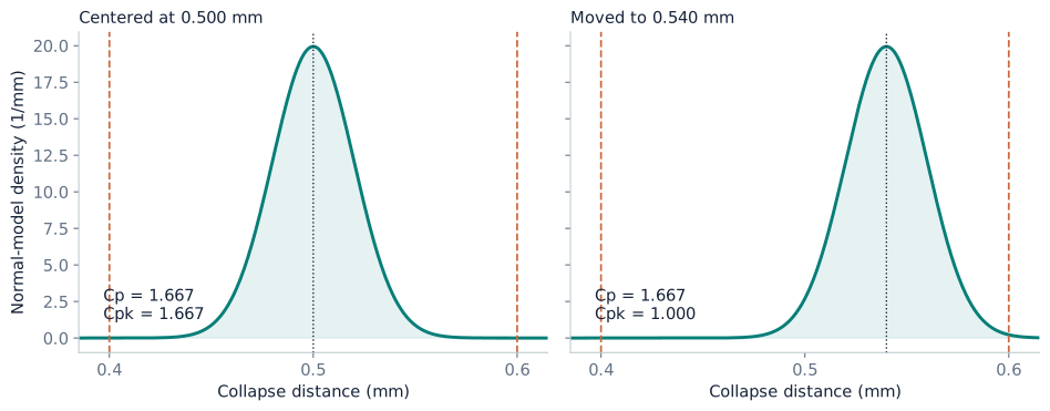
Start with a mean of 0.500 mm. It is 0.100 mm from either specification. Divide each distance by three within standard deviations, then take the smaller result.
CPL = (mean − LSL) / (3 × σ̂within) = 0.100 / 0.060 = 1.667
CPU = (USL − mean) / (3 × σ̂within) = 0.100 / 0.060 = 1.667
Cpk = min(CPL, CPU) = 1.667
Now move the mean to 0.540 mm and hold the standard deviation at 0.020 mm. The lower-side distance becomes 0.140 mm, while the upper-side distance shrinks to 0.060 mm. Cp remains 1.667 because the width and spread did not change.
CPL = 0.140 / 0.060 = 2.333
CPU = 0.060 / 0.060 = 1.000
Cpk = min(2.333, 1.000) = 1.000
Turn the comparison into an engineering explanation
The second process does not have a spread problem relative to the first. It has less upper-side room because its mean moved. A useful explanation is: “The within-based Cp is unchanged, but the upper specification limits Cpk because the mean is closer to USL.” That tells the team what to examine more clearly than simply writing “low capability.”
Recentring is a candidate action, not an automatic adjustment. The weld recipe may affect sealing, joint strength, alignment or another characteristic. Verify the cause and approved setting window before changing it. Then collect comparable subgroups and check that the intended correction persists.
Equal Cp and Cpk indicate centering at the tolerance midpoint under these two-sided definitions. They do not prove the process is on an engineering target that lies elsewhere. Nor do they establish statistical stability. A process can move over time even while a pooled capability result looks attractive.
For a normal-model interpretation, the distribution assumptions and stability evidence matter. A benchmark such as 1.33 is not universal authorization to release parts. State the required criterion, study design and uncertainty. The indices are dimensionless ratios, not a direct measurement of bond strength or a guarantee of zero future defects.
The takeaway
Cp answers the width-versus-spread question. Cpk adds the mean's distance to the nearer specification. Read them together: if Cp is much higher than Cpk, investigate centering; if both are low, examine variation as well as location.
References and calculation convention
This article uses the conventional within/overall definitions documented by Minitab, the average-range estimator and X̄–R factors in the NIST/SEMATECH handbook, and the ordinary overall sample standard deviation. The case and graphs are original illustrative calculations.