
The batch passes inspection, but its level changes
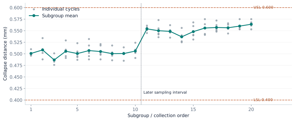
The engineer samples five consecutive cycles at each of twenty intervals: 100 measurements in total. Early windows sit near 0.500 mm; later windows are nearer 0.555 mm. Every sampled reading is inside 0.400–0.600 mm. We want to describe the spread across the whole collected study, including the separation between those windows.
Pp and Ppk use overall sample standard deviation. We can calculate them here and explain the observed collection, while limiting the interpretation: a changing sequence does not provide a stable model for predicting future output. Keep the time graph alongside the result.
The measurements and summary statistics
The downloadable table contains all twenty subgroups, five readings per row. The selected rows below show both ordinary within-window fluctuation and the later change in level. Values were rounded to 0.001 mm before calculation. A real measurement system still needs suitable resolution, repeatability and a defined displacement reference; recording three decimals alone establishes none of those properties.
| Group | Cycle 1 | Cycle 2 | Cycle 3 | Cycle 4 | Cycle 5 | Mean | Range |
|---|---|---|---|---|---|---|---|
| 1 | 0.501 | 0.500 | 0.510 | 0.497 | 0.496 | 0.5008 | 0.014 |
| 2 | 0.508 | 0.488 | 0.534 | 0.510 | 0.502 | 0.5084 | 0.046 |
| 9 | 0.485 | 0.514 | 0.502 | 0.500 | 0.502 | 0.5006 | 0.029 |
| 10 | 0.509 | 0.524 | 0.504 | 0.502 | 0.491 | 0.5060 | 0.033 |
| 11 | 0.551 | 0.556 | 0.557 | 0.561 | 0.545 | 0.5540 | 0.016 |
| 12 | 0.536 | 0.544 | 0.573 | 0.555 | 0.542 | 0.5500 | 0.037 |
| 19 | 0.553 | 0.560 | 0.558 | 0.554 | 0.575 | 0.5600 | 0.022 |
| 20 | 0.575 | 0.561 | 0.563 | 0.553 | 0.568 | 0.5640 | 0.022 |
Download all 20 subgroups or download the 100 observations in collection order. Both contain the same measurements in different layouts. Neither is a production benchmark.
N = 100 observations; k = 20 subgroups; n = 5 cycles per subgroup
LSL = 0.400 mm; USL = 0.600 mm; target = 0.500 mm
Grand mean x̄ = 0.52759 mm; average range R̄ = 0.03010 mm
Overall sample standard deviation = 0.02862121 mm
Retain full precision during intermediate calculations. The displayed results below are rounded for reading, so reproducing them from rounded standard deviations may produce a small last-digit difference. The full calculation uses the original three-decimal observations, not the rounded indices printed in the article.
Calculate overall sample standard deviation
Use every individual measurement, not just the twenty subgroup averages. There are N = 100 readings and their grand mean is 0.52759 mm. Subtract that mean from each reading, square the deviation, and add the 100 squared deviations. The total is 0.08109819 mm².
s = √[Σ(xᵢ − x̄)² / (N − 1)]
s = √(0.08109819 / 99) = 0.02862121 mm
The N − 1 denominator belongs to the sample estimate used here. Squared deviations have units of mm²; taking the square root returns millimetres. In Excel, STDEV.S applied to all 100 measurement cells produces the same result. Exclude subgroup labels, row means and ranges.
Pp uses the whole tolerance width
Pp = (USL − LSL) / (6s)
Pp = 0.200 / (6 × 0.02862121) ≈ 1.165
Like Cp, Pp ignores centering. It compares the available width with a six-standard-deviation reference spread. Here that spread includes the between-window change visible in the time graph. The name does not mean “a study lasting a particular number of days”; the overall estimator is what distinguishes this calculation.
Ppk includes the nearer specification
The mean's lower-side distance is 0.52759 − 0.400 = 0.12759 mm. Its upper-side distance is 0.600 − 0.52759 = 0.07241 mm. Three overall standard deviations equal approximately 0.08586363 mm.
PPL = 0.12759 / 0.08586363 ≈ 1.486
PPU = 0.07241 / 0.08586363 ≈ 0.843
Ppk = min(PPL, PPU) ≈ 0.843
The upper side limits the result. Pp is 1.165 while Ppk is 0.843 because the mean is above the specification midpoint. Those values describe the same data; one compares width, and the other accounts for the smaller upper margin. Keep full precision in calculations and round only the displayed result.
Why zero observed rejects does not contradict Ppk
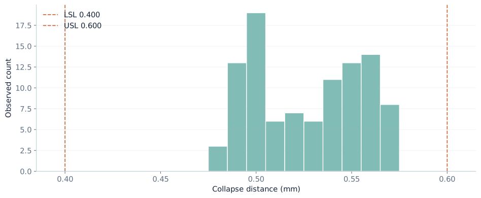
Inspection counted what happened in these 100 observations. The index compares the fitted spread and mean with the specifications. They answer different questions. The histogram shows two clusters, and the time graph shows their ordering. A single normal curve would not be a validated model of this changing process.
Do not turn Ppk 0.843 into a predicted reject rate for this case. A model-based probability requires justified distribution and process assumptions. Likewise, no observed rejects in a finite sample cannot establish zero future rejects. Report the count separately from the calculated index.
For one-sided specifications, calculate the appropriate upper or lower index. Do not invent an LSL to obtain Pp. Use the actual approved criteria and study conditions for acceptance, rather than treating any generic threshold as a release rule.
Reproduce this view
Download the data above and apply STDEV.S to all 100 readings, then use the three formulas. The browser trial demonstrates Pp/Ppk with 5–20 observations; its flat-data calculation uses overall sample standard deviation. It cannot take the complete 100-reading study.
The takeaway is to report both the estimator and the coverage of the study. Pp describes width against overall spread; Ppk adds centering.
References and calculation convention
This article uses the conventional within/overall definitions documented by Minitab, the average-range estimator and X̄–R factors in the NIST/SEMATECH handbook, and the ordinary overall sample standard deviation. The case and graphs are original illustrative calculations.