
Two reports from the same weld measurements
Twenty sampling windows contain five consecutive cycles each. The later windows sit higher than the earlier ones. The grand mean is 0.52759 mm; every observed reading is inside the example limits. A within-based calculation gives Cpk 1.865, while the overall-based calculation gives Ppk 0.843. Neither result uses different specifications or a different mean.
This article focuses on the reason for that gap. The calculations are descriptive illustrations because the collection contains a change. They do not establish a stable future process.
Within variation and overall variation
Each subgroup here consists of five consecutive cycles under a short window of similar conditions. Their range describes the spread inside that window. For equal subgroups of five, this example estimates within standard deviation using σ̂within = R̄ / d₂, with d₂ = 2.326. This is one established estimator; it is not the only possible within method.
Overall standard deviation is calculated from all 100 individual observations around their grand mean, using the sample denominator N − 1. The later observations sit farther from that grand mean because the process location moved. Their separation contributes to the overall spread even when consecutive cycles within each window remain fairly close together.
Do not calculate the overall standard deviation from just the 20 subgroup averages. That would describe the spread of averages, not the spread of the individual measured characteristic. Likewise, taking the standard deviation of the averages does not produce the within-cycle estimate needed for these Cp/Cpk formulas.
Subgroup formation therefore matters. Five consecutive cycles from one welder are different from five readings assembled from different machines or different hours. Mixing those streams can move variation into the wrong part of the calculation. Separate streams when their operating conditions justify it, and document any justified combined analysis.
Keep the numerator fixed and compare the denominators
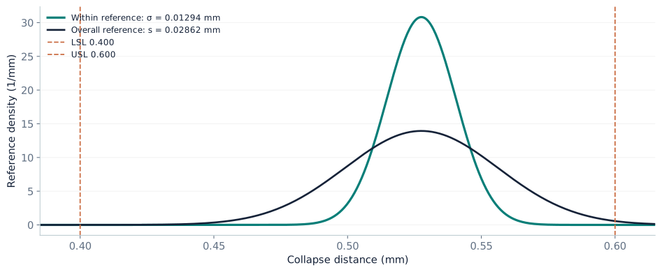
The twenty ranges average 0.03010 mm. For five-cycle subgroups, the range estimator gives σ̂within = 0.03010 / 2.326 = 0.01294067 mm. Overall sample standard deviation across the same 100 readings is 0.02862121 mm. The upper-side distance remains 0.07241 mm in both calculations.
Cpk = 0.07241 / (3 × 0.01294067) ≈ 1.865
Ppk = 0.07241 / (3 × 0.02862121) ≈ 0.843
Overall / within = 2.212; therefore Cpk / 2.212 ≈ Ppk
For completeness, the width-only results are Cp 2.576 and Pp 1.165. Both pairs change for the same reason: the overall denominator is wider. The local spread of consecutive cycles is smaller than the pooled spread that includes the separation between sampling windows.
Download the subgroup measurements. The estimator is R̄/d₂; using a pooled-standard-deviation estimator can change the within result. Match the method before comparing values across tools.
Why Cpk and Ppk differ here
The mean and nearest limit are identical in the two calculations. Only the denominator changes. Within sigma is 0.01294067 mm; overall standard deviation is 0.02862121 mm. The overall value is 2.212 times the within estimate, so Ppk is approximately Cpk divided by 2.212.
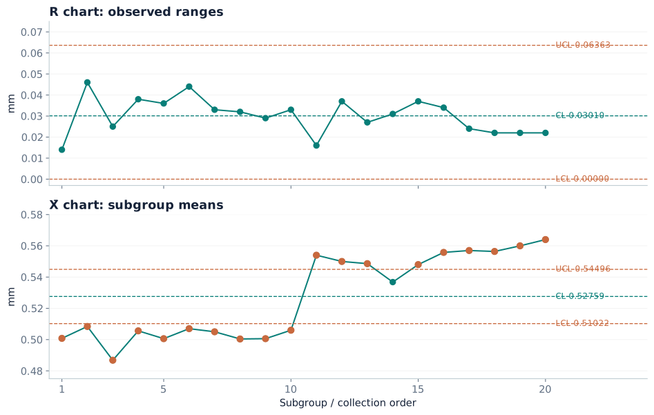
The time graph explains why. Later subgroup means sit at a higher level, making the combined observations wider around one grand mean. Within variation still describes the local spread of consecutive cycles. Cp/Cpk therefore show an attractive local-variation result while Pp/Ppk expose the poorer fit of the pooled study.
A gap is a prompt to examine time patterns, sampling, equipment streams and the chosen estimator. It is not a unique diagnosis of tool wear, operator error or any other cause. Nor is Ppk always mathematically required to be lower than Cpk in every finite sample. Estimator differences and sampling uncertainty can reverse a small gap.
A substantial difference should lead to evidence gathering. Do not automatically pick the higher value for release, or dismiss the lower value as “only long-term.” Report the study period and conditions behind both. The overall view describes this observed collection; it does not guarantee what the process will do tomorrow under different settings or materials.
Put the graphs back into the decision
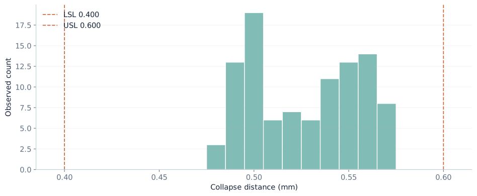
The histogram shows that every observed cycle is within the example specifications, but also suggests two levels. The collection-order graph shows when the level changed. A histogram loses this ordering: rearranging the same values produces the same histogram, mean and overall indices while potentially telling a very different operational story.
For a statistical check, calculate provisional X̄–R limits from all twenty subgroups. With n = 5, A₂ = 0.577, D₃ = 0 and D₄ = 2.114. The X̄ limits are 0.5102223 and 0.5449577 mm; the R limits are 0 and 0.0636314 mm. The range chart has no limit crossings, while the average chart shows multiple signals associated with the two levels.
These are not an approved production baseline. The presence of a change means the pooled normal-model capability results cannot establish stable future performance. You can calculate the indices and show them descriptively, as we did, while explicitly limiting the interpretation. Being able to calculate a result is different from having evidence to use it for release.
A useful investigation checks the displacement reference and measurement method, weld recipe history, tooling or fixture interventions, material and temperature records, and interruptions around the change. The graph does not confirm which occurred. If a cause is verified and corrected, mark the intervention and collect new comparable subgroups. Preserve the original record.
Read the gap as a clue, then check the sequence
A higher Cpk does not cancel the lower Ppk. Here, the local spread appears relatively small while the process level changes across the study. Report both estimates, retain the time ordering, and investigate the change.
References and calculation convention
This article uses the conventional within/overall definitions documented by Minitab, the average-range estimator and X̄–R factors in the NIST/SEMATECH handbook, and the ordinary overall sample standard deviation. The case and graphs are original illustrative calculations.